Using Formulas and Conditional Formatting to Track Tasks in Excel

Excel is an invaluable resource for effectively tracking completed tasks and pending work, particularly when working with repetitive, multi-step processes. Nevertheless, it can be tedious to mark every item, and overwhelming to figure out what’s already been done, and what work is left. Thankfully, this process can be automated using formulas and conditional formatting in Excel.

First, let’s look at how you could track a data migration – a somewhat messy, tedious process that requires exporting the data, mapping it to the columns in the new table, and cleaning up the data before even trying to get it into the new system.

This blog will review:

• How to use formulas to track the status of one field
• How to use formulas to track the status of an entity
• How to set conditional formatting based on the status of an entity

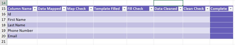
Specifically, the example table will show each field in an entity, if it maps to the field in a new entity, fills the import template, cleans the data, and how to show the entire table is complete using a cell outside the table.

Part of what makes these functions work is that they make use of structured references, which can only be done using tables. Without them, it requires constantly updating our functions as the table changes. To learn more about Excel tables, and how to set them up, check out this article.

Formulas

Is a Field Mapped?

Setting up a function to see whether you have finished mapping a specific field will include mapping the fields between the two entities, filling in the import template, and cleaning up the data. At each step you should check your work, to make sure the data is being imported accurately. (For this example, I created a table named “TableMap” below)

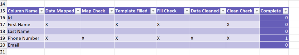
While checking off each completed task is a manual process, a formula can be used to check that everything is complete for a particular field:

IF(AND([@[Map Check]]="X",[@[Fill Check]]="X",[@[Clean Check]]="X"),1,0)

Let’s break down this formula to understand what is happening here.

Structured References

[@[Map Check]], [@[Fill Check]], and [@[Clean Check]] are all structured references – they all look for a specific cell in the table. The @ sign says that the formula should search for the cell in the row it’s in (the first row will find the cells in row 1, the second row will find the cells in row 2, etc.) The name in the inner square brackets is the name of the column to look for.

In this case, the formula looks at the values in the current row, in the “Map Check,” “Fill Check,” and “Clean Check” columns.

You can set a structured reference either by clicking the cell you want to use when building the formula, or by typing the reference in.

AND(test 1[, test 2] [, test 3…])

The AND() function takes one or more logical expressions and evaluates whether or not all of the given expressions are true. In our case, the AND() function will return true if and only if the Map Check, Fill Check, and Clean Check columns all have the value “X”.

IF(Expression, [True,] [False])

The IF() function will take in a logical expression, evaluate it, and return one value if the expression is true and another if the expression is false. If you don’t specify the values to return, it will provide a Boolean that is either TRUE or FALSE.

Together, the whole function will evaluate whether the Map Check, Fill Check, and Clean Check fields are all “X.” If they are, it will return a 1, and if they aren’t, it will return a 0.

Note: This function only looks at specific cells and values. If you want to use other symbols if you check a cell but there’s an issue, such as a “-,” or if you want to add in columns that don’t need to be filled, like a Notes column, this function will still work as intended.

Set Completion Status

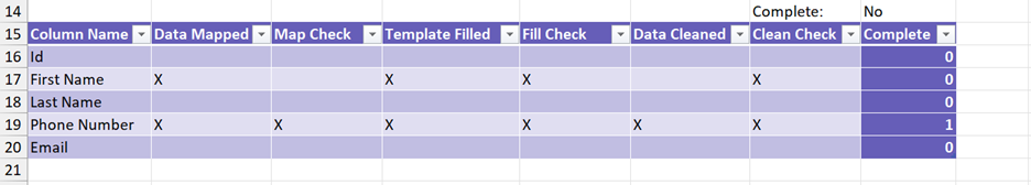
Now you can see if your fields are done and easily tell if there’s only a few fields to work on. However, what if you have too many fields to manage? Rather than needing to scroll through a long table to see what is missing, another formula can immediately show if you have finished preparing that entity for import:

=IF(COUNTIF(TableMap[Complete],1)=ROWS(TableMap), “Yes”, “No”)

Note: Since the formula is outside of the table, you need to use the table’s name to get data from it. If you don’t give your table a name, it defaults to Table1, Table 2, etc.

COUNTIF(range, criteria)

COUNTIF() checks how many cells in the selected range match the given criteria. In this formula, it’s checking the Complete column and returning the count of cells that have the value 1. In other words, it shows how many fields are fully prepared for import.

ROWS()

The ROWS() function returns how many rows are in the given array or table. In this case, it shows how many fields in total need to be prepared for import.

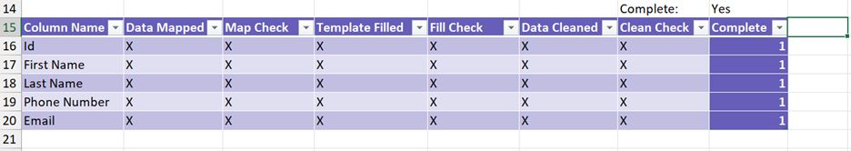
In this function, the IF() function is used to check whether the COUNTIF() and ROWS() values are the same. Once it’s checked, it will output “Yes” if they’re equal, and “No” if they’re not. In other words, this function answers the question “Am I done?”

Note: For this example, everything is on one sheet. However, we can also use this same formula in other sheets. If you set up this table for every entity you need to map (just by duplicating the table or its sheet,) you can then see the status of all your entities in one place.

Conditional Formatting

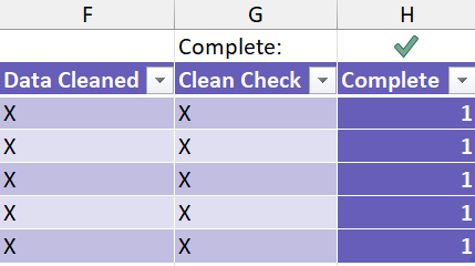
What if you’d rather use visuals to see the status of your entities? Well, with conditional formatting, you can change the format of a cell or add icons to represent different cell values.

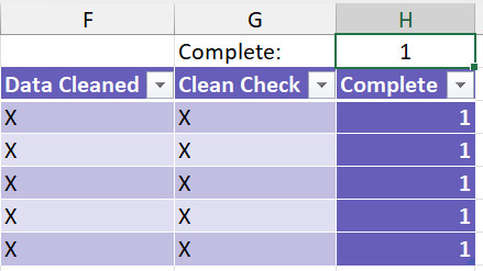
First, you’ll need to make an adjustment to the “is-my-entity-ready” formula. Instead of returning “Yes” or “No,” it’s going to return 1 or 0:

IF(COUNTIF(TableMap[Complete],1)=ROWS(TableMap[Complete]),1,0)

This will make it easier to set up the conditional formatting.

How to Set Conditional Formatting

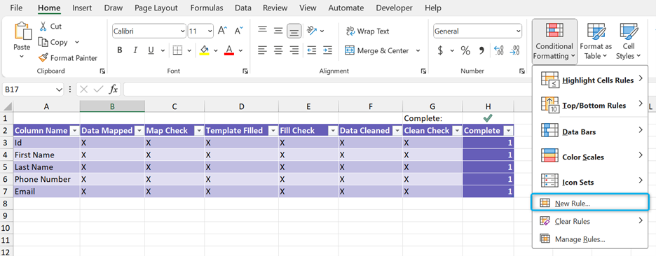
1. Select the cell (or range of cells) you want to apply the formatting to. (Note: You can change this later.)
   
2. Open the “Home” tab in Excel, click “Conditional Formatting,” and click “New Rule…”
   
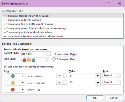
3. Ensure you select the rule type “Format all cells based on their values”. In the “Edit the Rule Description” section, change “Format Style” to “Icon Sets”.
   
4. Set the Icon Style, or just set the individual icons later.
   1. If you only want to see the icon, check “Show Icon Only”.
5. Change the “Type” to “Number” for the first and second conditions and set the values to 1 and 0 respectively.
   1. If you don’t like the set of icons from the Icon Style, click the icon next to the condition you want to change and select the desired icon.
      

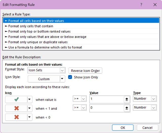
Note: This rule is essentially saying “If the value in the cell is greater than or equal to the number 1, then use the checkmark icon. Otherwise, if it’s less than 1 and greater than or equal to 0, set it to an X.” Since the icon sets are based on three possible values, but the cell this is used on can only be 1 or 0, the third condition simply isn’t being used here.

6. Click “OK”.

If set up correctly, you should now see the icon either in place of or next to the entity’s status.

If you want to modify this formatting rule later, or change what cells it affects, click “Conditional Formatting” and select “Manage Rules.” From there, you can change any existing rules.

Summary

Tasks like preparing data for data migration are as important as they are difficult to manage. Fortunately, Excel can make managing and tracking data easier. TopLine Results specializes in data management tasks like this. We've helped customers set up and manage CRM software like Microsoft Dynamics, Zoho, Act! and HubSpot. If you need assistance managing your CRM or its data, contact us at 800-880-1960 or info@toplineresults.com to learn more.